Simple Visualisations and Examples

Examples and Explanations

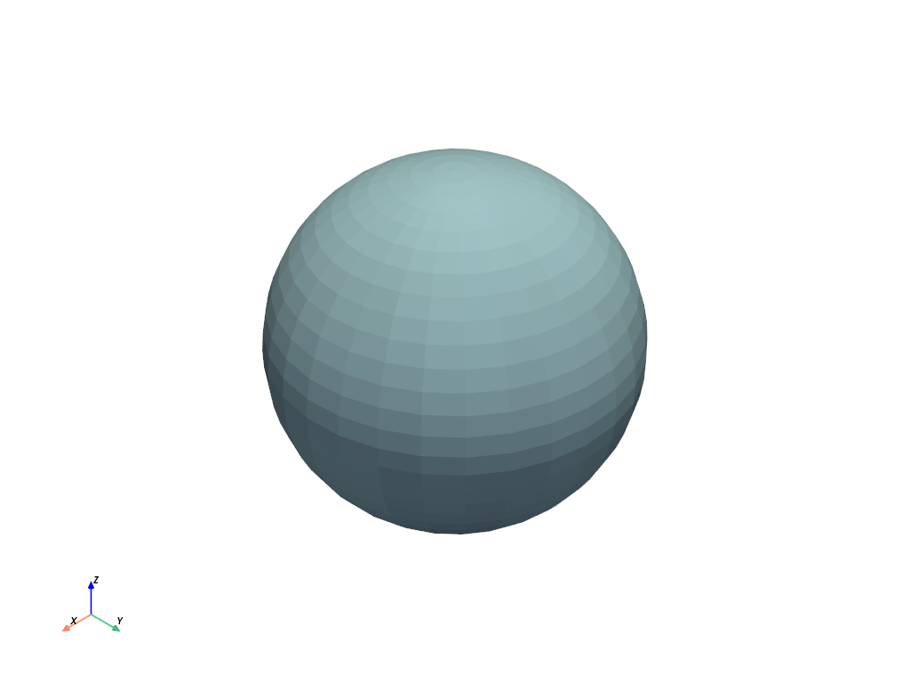
After the installation, we can start using PyVista for 3D visualization. Here area some simple examples to plot and analyse 3D mesh:

We will start with a simple 3 dimensional sphere.

import pyvista as pv

# Create a simple mesh (sphere)
sphere = pv.Sphere()

# Plot the mesh
sphere.plot()

Use a topographic surface to create a 3D terrain-following mesh. In this example, we demonstrate a simple way to make a 3D grid/mesh that follows a given topographic surface.

from pyvista import examples

mesh = examples.load_random_hills() # automatically download
contours = mesh.contour()
contours

Header	Data Arrays
PolyData Information N Cells 3709 N Points 3731 N Strips 0 X Bounds -1.000e+01, 1.000e+01 Y Bounds -2.309e-14, 2.000e+01 Z Bounds 9.573e-01, 7.483e+00 N Arrays 2	Name Field Type N Comp Min Max Normals Points float32 3 -8.643e-01 9.992e-01 Elevation Points float32 1 9.573e-01 7.483e+00

mesh.plot()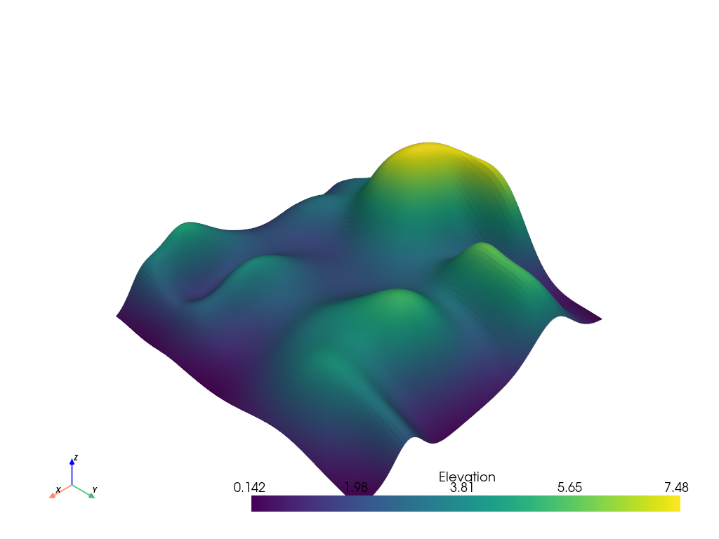

If you have a structured dataset like a pyvista.ImageData or pyvista.RectilinearGrid, you can clip it using the pyvista.Plotter.add_volume_clip_plane() widget to better see the internal structure of the dataset.

import numpy as np

import pyvista as pv

grid = pv.ImageData(dimensions=(200, 200, 200))
grid['scalars'] = np.linalg.norm(grid.center - grid.points, axis=1)
grid

Header	Data Arrays
ImageData Information N Cells 7880599 N Points 8000000 X Bounds 0.000e+00, 1.990e+02 Y Bounds 0.000e+00, 1.990e+02 Z Bounds 0.000e+00, 1.990e+02 Dimensions 200, 200, 200 Spacing 1.000e+00, 1.000e+00, 1.000e+00 N Arrays 1	Name Field Type N Comp Min Max scalars Points float64 1 8.660e-01 1.723e+02

opacity = np.zeros(100)
opacity[::10] = np.geomspace(0.01, 0.75, 10)

pl = pv.Plotter()
pl.add_volume_clip_plane(grid, normal='-x', opacity=opacity[::-1], cmap='magma')
pl.show()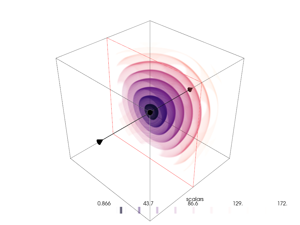

import numpy as np
import pyvista

rng = np.random.default_rng(seed=0)
point_cloud = rng.random((100, 3))
pdata = pyvista.PolyData(point_cloud)
pdata['orig_sphere'] = np.arange(100)

# create many spheres from the point cloud
sphere = pyvista.Sphere(radius=0.02, phi_resolution=10, theta_resolution=10)
pc = pdata.glyph(scale=False, geom=sphere, orient=False)
pc.plot(cmap='Reds')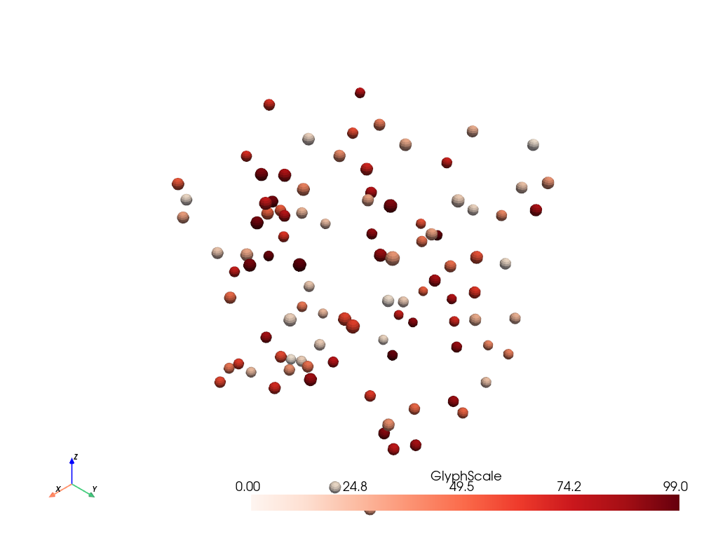

Performing boolean/topological operations (intersect, union, difference) methods are implemented for pyvista.PolyData mesh types only and are accessible directly from any pyvista.PolyData mesh.

import pyvista
import numpy as np

def make_cube():
    x = np.linspace(-0.5, 0.5, 25)
    grid = pyvista.StructuredGrid(*np.meshgrid(x, x, x))
    surf = grid.extract_surface().triangulate()
    surf.flip_normals()
    return surf

# Create example PolyData meshes for boolean operations
sphere = pyvista.Sphere(radius=0.65, center=(0, 0, 0))
cube = make_cube()

# Perform a boolean difference
boolean = cube.boolean_difference(sphere)
boolean.plot(color='darkgrey', smooth_shading=True, split_sharp_edges=True)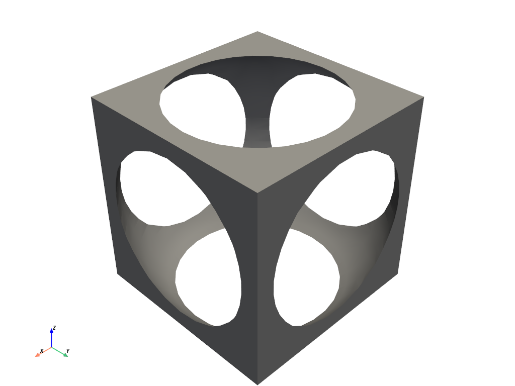

Creating a spline/polyline from a numpy array of XYZ vertices using pyvista.Spline().

import numpy as np
import pyvista

# Make the xyz points
theta = np.linspace(-10 * np.pi, 10 * np.pi, 100)
z = np.linspace(-2, 2, 100)
r = z**2 + 1
x = r * np.sin(theta)
y = r * np.cos(theta)
points = np.column_stack((x, y, z))

spline = pyvista.Spline(points, 500).tube(radius=0.1)
spline.plot(scalars='arc_length', show_scalar_bar=False)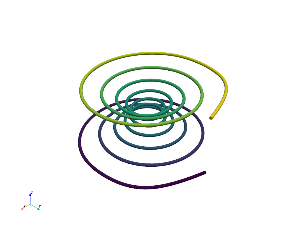

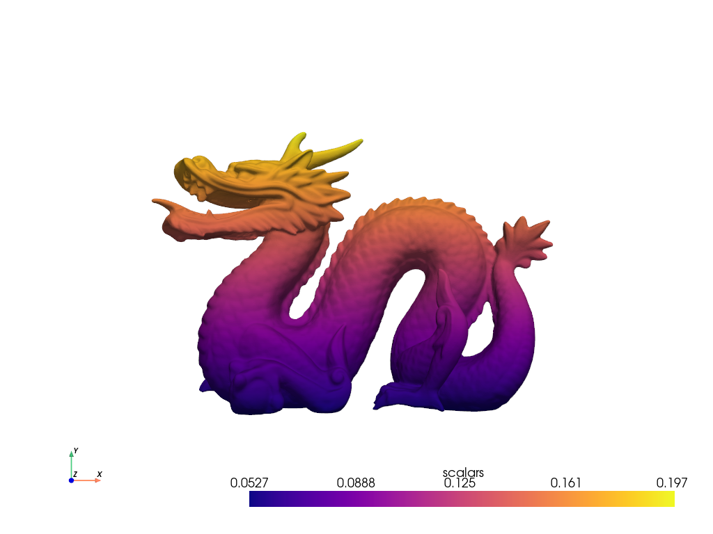
Here, we download the Stanford dragon mesh, color it according to height, and plot it using a web-viewer.

from pyvista import examples
mesh = examples.download_dragon()
mesh['scalars'] = mesh.points[:, 1]
mesh.plot(cpos='xy', cmap='plasma')